Much of the world’s data is locked in PDFs, JPEGs, and other documents. Traditional OCR extracts text but loses critical information: the layout of tables with merged cells, the relationship between charts and captions, the reading order of multi-column layouts, etc.
Inspired by the Document AI: From OCR to Agentic Doc Extraction course from DeepLearning.AI, I built a comprehensive system that processes documents the way humans do: breaking them into parts, examining each piece carefully, and extracting information through multiple iterations using AI agents.
This blog post walks through building an agentic document understanding system that combines OCR, layout detection, reading order analysis, and visual language models to create intelligent document processing pipelines.
The Challenge
When processing complex documents like research papers, invoices, or reports, we face several challenges:
- Text extraction: OCR can extract text, but loses spatial relationships
- Layout understanding: Tables, charts, and multi-column layouts need special handling
- Reading order: Documents aren’t always read top-to-bottom, left-to-right
- Context preservation: Charts need their captions, tables need their headers
- Structured extraction: Converting unstructured documents into queryable formats
The Solution: A Multi-Stage Pipeline
Our system processes documents through several stages:
- PDF to Images: Convert PDF pages to PIL images for processing
- OCR Extraction: Use PaddleOCR to extract text with bounding boxes
- Reading Order: Use LayoutReader to determine logical reading sequence
- Layout Detection: Identify different regions (text, tables, figures, titles)
- Region Cropping: Extract specific regions for focused analysis
- VLM Analysis: Use Gemini’s vision capabilities to analyze charts and tables
- Agent Assembly: Build an AI agent that can intelligently query the document
Here’s a detailed walkthrough of each step.
Step 1: Setup and PDF Conversion
We start by installing the necessary dependencies and converting our PDF into images:
!pip install paddlepaddle==3.2.0 paddleocr==3.3.3
!pip install langchain==0.0.350
!apt-get install poppler-utils
!pip install pdf2image

import os
from PIL import Image
from pathlib import Path
from typing import List, Dict, Any, Optional
import numpy as np
from pdf2image import convert_from_path

# Convert PDF to PIL images
PDF_FILE_PATH = Path("2108.11591v2.pdf")
all_pil_images = convert_from_path(PDF_FILE_PATH, dpi=200)
print(f"Converted {len(all_pil_images)} pages from PDF")
Converting PDFs to images allows us to process each page as a visual object, preserving layout information that would be lost in pure text extraction.
Step 2: OCR with PaddleOCR
PaddleOCR is a powerful open-source OCR tool that provides both text extraction and bounding box coordinates:
from paddleocr import PaddleOCR

# Initialize OCR
ocr = PaddleOCR(use_angle_cls=True, lang='en')

# Run OCR on all pages
all_ocr_results = []
for i, pil_image_for_ocr in enumerate(all_pil_images):
    print(f"Processing page {i+1}/{len(all_pil_images)}...")
    result = ocr.predict(np.array(pil_image_for_ocr))
    all_ocr_results.append(result[0])
PaddleOCR returns structured results with:
- Text: The extracted text content
- Bounding boxes: Coordinates for each text region
- Confidence scores: How certain the model is about each detection
Step 3: Visualizing OCR Results
To understand what OCR extracted, we visualize the bounding boxes:
import cv2
import matplotlib.pyplot as plt

# For demonstration, let's still show the results for the page
page = all_ocr_results[3]
current_texts = page['rec_texts']
current_scores = page['rec_scores']
current_boxes = page['rec_polys']
current_processed_img = page['doc_preprocessor_res']['output_img']

print(f"Extracted {len(current_texts)} text regions for the page.")
print("First 15 extracted texts and their confidence scores:")
for text, score in list(zip(current_texts, current_scores))[:15]:
    print(f"  {text!r:45} | {score:.3f}")

img_plot = current_processed_img.copy()
show_text= False

for text, box in zip(current_texts, current_boxes):
    pts = np.array(box, dtype=int)
    cv2.polylines(img_plot, [pts], True, (0, 255, 0), 2)
    x, y = pts[0]
    if show_text:
        cv2.putText(img_plot, text, (x, y - 5),
                    cv2.FONT_HERSHEY_SIMPLEX, 0.6, (255, 0, 0), 2)

plt.figure(figsize=(8, 10))
plt.imshow(cv2.cvtColor(img_plot, cv2.COLOR_BGR2RGB))
plt.axis("off")
plt.title("Aligned Bounding Boxes (Processed Image)")
plt.show()
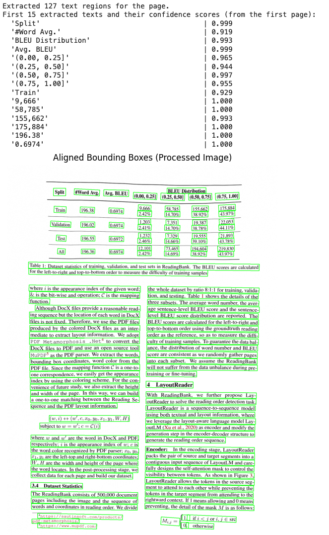
This visualization helps us verify that OCR correctly identified text regions and understand the spatial distribution of content.
Step 4: Structuring OCR Results
We create a dataclass to structure OCR results for easier processing:
from dataclasses import dataclass

@dataclass
class OCRRegion:
    text: str
    bbox: list
    confidence: float

    @property
    def bbox_xyxy(self):
        x_coords = [p[0] for p in self.bbox]
        y_coords = [p[1] for p in self.bbox]
        return [min(x_coords), min(y_coords), max(x_coords), max(y_coords)]

ocr_regions: List[OCRRegion] = []

for page_result in all_ocr_results:
    page_texts = page_result['rec_texts']
    page_scores = page_result['rec_scores']
    page_boxes = page_result['rec_polys']

    for text, score, box in zip(page_texts, page_scores, page_boxes):
        ocr_regions.append(OCRRegion(text=text, bbox=box.astype(int).tolist(), confidence=score))

print(f"Stored {len(ocr_regions)} OCR regions from all pages.")
This structured format makes it easier to combine OCR results with layout detection and reading order information.
Step 5: Reading Order Detection with LayoutReader
Simple ordering (e.g., top-to-bottom, left-to-right) does not apply to our complex document. We will use LayoutReader, which itself utilizes the LayoutLMv3 model (available on Hugging Face). Additionally, we use helper functions for LayoutReader available in this repository: ppaanngggg/layoutreader/helpers.py.
!pip install transformers
from transformers import LayoutLMv3ForTokenClassification

# Load LayoutReader model
print("Loading LayoutReader model...")
model_slug = "hantian/layoutreader"
layout_model = LayoutLMv3ForTokenClassification.from_pretrained(model_slug)
print("Model loaded successfully!")

def get_reading_order(ocr_regions):
    max_x = max_y = 0
    for region in ocr_regions:
        x1, y1, x2, y2 = region.bbox_xyxy
        max_x, max_y = max(max_x, x2), max(max_y, y2)
    image_width, image_height = max_x * 1.1, max_y * 1.1

    boxes = []
    for region in ocr_regions:
        x1, y1, x2, y2 = region.bbox_xyxy
        left = int((x1 / image_width) * 1000)
        top = int((y1 / image_height) * 1000)
        right = int((x2 / image_width) * 1000)
        bottom = int((y2 / image_height) * 1000)
        boxes.append([left, top, right, bottom])

    inputs = boxes2inputs(boxes)
    inputs = prepare_inputs(inputs, layout_model)
    logits = layout_model(**inputs).logits.cpu().squeeze(0)
    return parse_logits(logits, len(boxes))

reading_order = get_reading_order(ocr_regions)
print(f"Reading order: {reading_order[:20]}...")
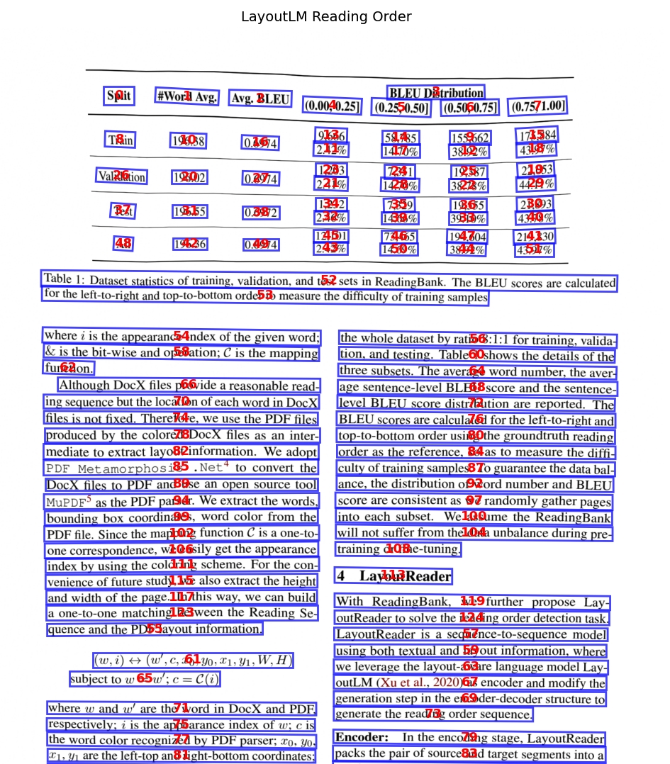
LayoutReader uses both textual and layout information to determine the logical sequence in which humans would read the document. This is crucial for maintaining context when processing multi-column layouts or complex structures.
Step 6: Visualizing the Reading Order
Visualize reading order with numbered overlays on each region. Numbers follow the predicted reading sequence.
import matplotlib.patches as patches

def visualize_reading_order(ocr_regions, image_array, reading_order, title="Reading Order"):
    """
    Visualize OCR regions with their reading order numbers using matplotlib.
    """

    fig, ax = plt.subplots(1, figsize=(10, 14))
    ax.imshow(cv2.cvtColor(image_array, cv2.COLOR_BGR2RGB))

    # Create order mapping: index -> reading order position
    order_map = {i: order for i, order in enumerate(reading_order)}

    for i, region in enumerate(ocr_regions):
        bbox = region.bbox
        if bbox and len(bbox) >= 4:
            # Draw polygon
            ax.add_patch(patches.Polygon(bbox, linewidth=2,
                                         edgecolor='blue',
                                         facecolor='none', alpha=0.7))
            # Add reading order number at center
            xs = [p[0] for p in bbox]
            ys = [p[1] for p in bbox]
            ax.text(sum(xs)/len(xs), sum(ys)/len(ys),
                    str(order_map.get(i, i)),
                    fontsize=13, color='red',
                    ha='center', va='center', fontweight='bold')

    ax.set_title(title, fontsize=14)
    ax.axis('off')
    plt.tight_layout()
    plt.show()

# Get the processed image from OCR results for visualization
# Note: If you processed a specific page (e.g., page 3), use the corresponding index
page = all_ocr_results[0]  # Adjust index based on which page you processed
current_processed_img = page['doc_preprocessor_res']['output_img']
img_plot = current_processed_img.copy()

visualize_reading_order(ocr_regions, img_plot,
                        reading_order, "LayoutLM Reading Order")
Step 7: Combining OCR Text with Reading Order
With the reading order determined, we combine the OCR text with this sequence to create a structured output of ordered text:
def get_ordered_text(ocr_regions, reading_order):
    indexed = [(reading_order[i], i, ocr_regions[i]) for i in range(len(ocr_regions))]
    indexed.sort(key=lambda x: x[0])
    return [
        {"position": pos, "text": r.text, "confidence": r.confidence, "bbox": r.bbox_xyxy}
        for pos, _, r in indexed
    ]

current_ordered_text = get_ordered_text(ocr_regions, reading_order)
print("Ordered text (first 10 items):")
for item in current_ordered_text[:10]:
    print(f"  [{item['position']}] {item['text']}")
This ordered text representation maintains the logical flow of the document, making it easier for LLMs to understand context and relationships.
Step 8: Layout Detection
After extracting the ordered text, we perform layout detection on all pages to identify different structural regions (e.g., text, title, table, figure, chart). This step structures the document content by recognizing different element types.
from paddleocr import LayoutDetection

# Initialize layout detection
layout_engine = LayoutDetection()

# Perform layout detection on all PIL images. This returns a list of results, one for each page.
all_layout_detection_results = layout_engine.predict(np.array(all_pil_images))

print(f"Successfully performed layout detection on {len(all_layout_detection_results)} pages.")
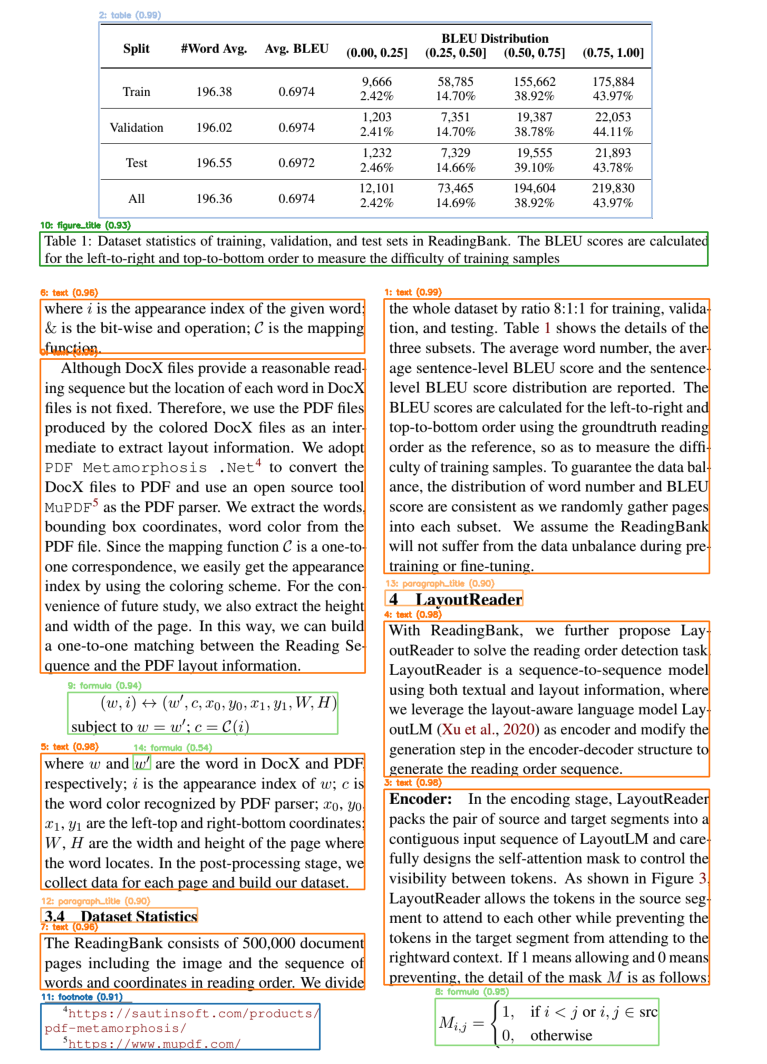
Layout detection enables us to:
- Identify tables for structured data extraction
- Find figures and charts for visual analysis
- Separate titles from body text for hierarchical understanding
- Detect formulas that need special processing
Step 9: Structuring Layout Regions
Having obtained layout detection results for all pages, we structure these results into LayoutRegion dataclass objects. This provides a standardized and accessible format for further processing and visualization of the layout information.
@dataclass
class LayoutRegion:
    region_id: int
    region_type: str
    bbox: list  # [x1, y1, x2, y2]
    confidence: float
    page_idx: int # Added page_idx to the dataclass

# Store layout regions in structured format
all_layout_regions: List[LayoutRegion] = []
page_offset = 0

for page_idx, page_layout_results in enumerate(all_layout_detection_results):
    current_regions = []
    for box_id, box_data in enumerate(page_layout_results['boxes']):
        current_regions.append(LayoutRegion(
            region_id=page_offset + box_id,
            region_type=box_data['label'],
            bbox=[int(x) for x in box_data['coordinate']],
            confidence=box_data['score'],
            page_idx=page_idx # Populate page_idx here
        ))
    # Sort regions by their Y-coordinate for better readability
    current_regions.sort(key=lambda r: r.bbox[1])
    all_layout_regions.extend(current_regions)
    page_offset += len(page_layout_results['boxes'])

print(f"Stored {len(all_layout_regions)} layout regions from all pages.")
# Display first few structured regions for verification
print("First 5 structured layout regions:")
for i, region in enumerate(all_layout_regions[:5]):
    print(f"  Region ID: {region.region_id}, Type: {region.region_type}, Confidence: {region.confidence:.2f}, BBox: {region.bbox}, Page: {region.page_idx}")
Step 10: Visualizing Layout Detection
Visualize layout regions with color-coded boxes showing region ID, type, and confidence.
# Visualize layout detection
from matplotlib import colormaps

def visualize_layout(image_array, layout_regions, min_confidence=0.5,
                     title="Layout Detection"):
    """
    Visualize layout detection results using cv2 (same pattern as L2).
    """
    img_plot = image_array.copy()

    # Get unique labels and generate colors
    labels = list(set(r.region_type for r in layout_regions))
    cmap = colormaps.get_cmap('tab20')
    color_map = {}
    for i, label in enumerate(labels):
        rgba = cmap(i % 20)
        color_map[label] = (int(rgba[2]*255), int(rgba[1]*255), int(rgba[0]*255))

    for region in layout_regions:
        if region.confidence < min_confidence:
            continue

        color = color_map[region.region_type]
        x1, y1, x2, y2 = region.bbox

        # Draw rectangle
        pts = np.array([[x1, y1], [x2, y1], [x2, y2], [x1, y2]], dtype=int)
        cv2.polylines(img_plot, [pts], True, color, 2)

        # Add label
        text = f"{region.region_id}: {region.region_type} ({region.confidence:.2f})"
        cv2.putText(img_plot, text, (x1, y1-8),
                    cv2.FONT_HERSHEY_SIMPLEX, 0.5, color, 2)

    plt.figure(figsize=(12, 16))
    plt.imshow(cv2.cvtColor(img_plot, cv2.COLOR_BGR2RGB))
    plt.axis("off")
    plt.title(title)
    plt.show()

    return img_plot

img_plot = np.array(all_pil_images[3]).copy()
# Visualize layout regions for page 3
visualize_layout(img_plot,
                 [region for region in all_layout_regions if region.page_idx == 3],
                 min_confidence=0.5,
                 title="Page 3 Layout Detection")
Step 11: Cropping Regions for VLM Analysis
For focused analysis of specific regions (like tables or charts), we crop them from the full page and convert them to base64 for VLM processing:
from io import BytesIO
import base64

def crop_region(pil_image: Image.Image, bbox: list, padding: int = 5) -> Image.Image:
    """Crop a region from a PIL image using bounding box coordinates.

    Args:
        pil_image: PIL Image to crop from
        bbox: Bounding box as [x1, y1, x2, y2]
        padding: Padding to add around the bounding box
    """
    # bbox is [x1, y1, x2, y2]
    x1, y1, x2, y2 = bbox

    x1 = max(0, x1 - padding)
    y1 = max(0, y1 - padding)
    x2 = min(pil_image.width, x2 + padding)
    y2 = min(pil_image.height, y2 + padding)

    return pil_image.crop((x1, y1, x2, y2))

def image_to_base64(img: Image.Image) -> str:
    """Convert PIL Image to base64 string."""
    buf = BytesIO()
    img.save(buf, format="PNG")
    return base64.b64encode(buf.getvalue()).decode("utf-8")

# Store cropped regions with base64 encoding
region_images: Dict[str, Dict] = {}

# Group layout regions by page for easier processing
regions_by_page = {i: [] for i in range(len(all_pil_images))}
for region in all_layout_regions:
    regions_by_page[region.page_idx].append(region)

# for page_idx, pil_image in enumerate(all_pil_images):
for page_idx, pil_image in enumerate([all_pil_images[3]]):
    page_layout_regions = regions_by_page[page_idx]
    print(f"Processing page {page_idx} with {len(page_layout_regions)} regions...")

    for region in page_layout_regions:
        cropped = crop_region(pil_image, region.bbox)
        region_key = f"page_{page_idx}_region_{region.region_id}"
        region_images[region_key] = {
            "image": cropped,
            "base64": image_to_base64(cropped),
            "type": region.region_type,
            "bbox": region.bbox,
            "page_idx": region.page_idx # Use the correct page_idx from the region object
        }

print(f"Cropped {len(region_images)} regions from all pages; full image base64 ready.")
Cropping regions provides several benefits:
- Focused analysis: VLM sees only relevant content
- Reduced noise: No surrounding text interference
- Lower costs: Smaller images reduce API costs
- Better accuracy: Models perform better on focused content
Step 12: Creating VLM Tools with Gemini
We create specialized tools that use Gemini’s vision capabilities to analyze tables and charts. We begin by defining the analysis prompts and a helper function:
from google import genai
from google.genai import types
from google.colab import userdata

os.environ['GOOGLE_API_KEY'] = userdata.get('GOOGLE_API_KEY')

# Create Gemini client (will automatically pick up GOOGLE_API_KEY or GEMINI_API_KEY from env)
client = genai.Client()

# Define prompts for chart and table analysis
CHART_ANALYSIS_PROMPT = """You are a Chart Analysis specialist.
Analyze this chart/figure image and extract:

1. **Chart Type**: (line, bar, scatter, pie, etc.)
2. **Title**: (if visible)
3. **Axes**: X-axis label, Y-axis label, and tick values
4. **Data Points**: Key values (peaks, troughs, endpoints)
5. **Trends**: Overall pattern description
6. **Legend**: (if present)

Return a JSON object with this structure:
{
  "chart_type": "...",
  "title": "...",
  "x_axis": {"label": "...", "ticks": [...]},
  "y_axis": {"label": "...", "ticks": [...]},
  "key_data_points": [...],
  "trends": "...",
  "legend": [...]
}
"""

TABLE_ANALYSIS_PROMPT = """You are a Table Extraction specialist.
Extract structured data from this table image.

1. **Identify Structure**:
    - Column headers, row labels, data cells
2. **Extract All Data**:
    - Preserve exact values and alignment
3. **Handle Special Cases**:
    - Merged cells, empty cells (mark as null), multi-line headers

Return a JSON object with this structure:
{
  "table_title": "...",
  "column_headers": ["header1", "header2", ...],
  "rows": [
    {"row_label": "...", "values": [val1, val2, ...]},
    ...
  ],
  "notes": "any footnotes or source info"
}
"""

# Helper function to call VLM with base64 image
def call_vlm_with_image(image_base64: str, prompt: str) -> str:
    """Call Gemini VLM with a base64-encoded image and prompt."""
    import base64
    # Decode base64 image to bytes
    image_bytes = base64.b64decode(image_base64)
    # Create Part from bytes using the SDK
    image_part = types.Part.from_bytes(data=image_bytes, mime_type="image/png")
    # Generate content with Gemini using the client
    response = client.models.generate_content(
        model="gemini-2.5-flash",
        contents=[prompt, image_part]
    )
    return response.text
Here’s an example using a region that contains a table:
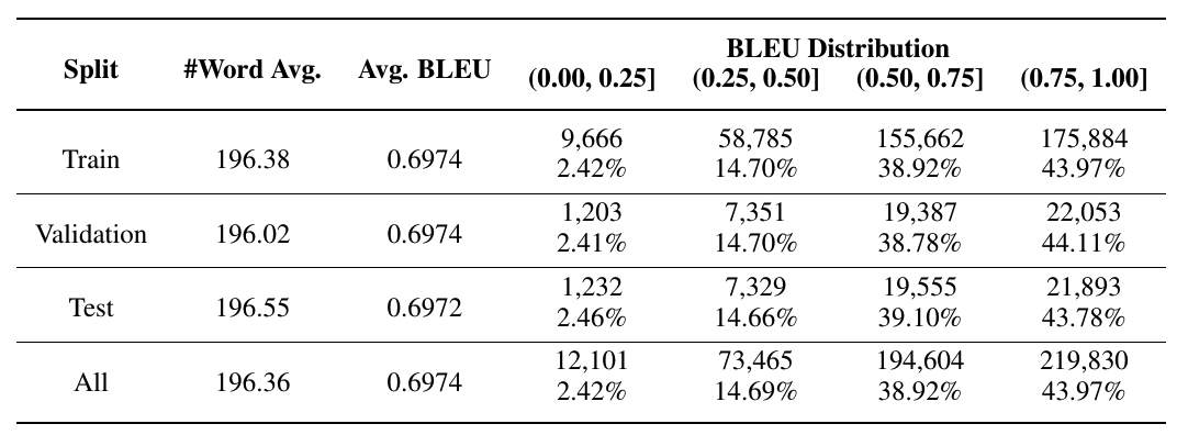
# Example using a region that contains a table
table_image_base64 = region_images['page_3_region_1']['base64']

vlm_raw = call_vlm_with_image(table_image_base64, TABLE_ANALYSIS_PROMPT)
print(vlm_raw[:800])
{
  "table_title": null,
  "column_headers": [
    "Split",
    "#Word Avg.",
    "Avg. BLEU",
    "BLEU Distribution (0.00, 0.25]",
    "BLEU Distribution (0.25, 0.50]",
    "BLEU Distribution (0.50, 0.75]",
    "BLEU Distribution (0.75, 1.00]"
  ],
  "rows": [
    {
      "row_label": "Train",
      "values": [
        "196.38",
        "0.6974",
        "9,666\n2.42%",
        "58,785\n14.70%",
        "155,662\n38.92%",
        "175,884\n43.97%"
      ]
    },
    {
      "row_label": "Validation",
      "values": [
        "196.02",
        "0.6974",
        "1,203\n2.41%",
        "7,351\n14.70%",
        "19,387\n38.78%",
        "22,053\n44.11%"
      ]
    },
    {
      "row_label": "Test",
      "values": [
        "196.55",
        "0.6972",
        "1,232\n2.46%",
        "7,329\n14.66%",
        "19,555\n39.10%",
        "21,893\n43.78%"
      ]
    },
    {
      "row_label": "All",
      "values": [
        "196.36",
        "0.6974",
        "12,101\n2.42%",
        "73,465\n14.69%",
        "194,604\n38.92%",
        "219,830\n43.97%"
      ]
    }
  ],
  "notes": null
}
Next, we define the analysis tools:
def analyze_chart_tool(region_id: int) -> str:
    """Analyze a chart or figure region using VLM.
    Use this tool when you need to extract data from charts, graphs, or figures.

    Args:
        region_id: The ID of the layout region to analyze (must be a chart/figure type)

    Returns:
        JSON string with chart type, axes, data points, and trends
    """
    if region_id not in region_images:
        return f"Error: Region {region_id} not found. Available regions: {list(region_images.keys())}"

    region_data = region_images[region_id]

    if region_data['type'] not in ['chart', 'figure']:
        return f"Warning: Region {region_id} is type '{region_data['type']}', not a chart/figure. Proceeding anyway."

    result = call_vlm_with_image(region_data['base64'], CHART_ANALYSIS_PROMPT)

    return result

def analyze_table_tool(region_id: int) -> str:
    """
    Extract structured data from a table region using VLM.
    Use this tool when you need to extract tabular data
    with headers and rows.

    Args:
        region_id: The ID of the layout region to analyze (must be a table type)

    Returns:
        JSON string with table headers, rows, and any notes
    """
    if region_id not in region_images:
        return f"Error: Region {region_id} not found. Available regions: {list(region_images.keys())}"

    region_data = region_images[region_id]

    if region_data['type'] != 'table':
        return f"Warning: Region {region_id} is type '{region_data['type']}', not a table. Proceeding anyway."

    result = call_vlm_with_image(region_data['base64'], TABLE_ANALYSIS_PROMPT)
    return result
These tools enable the agent to intelligently analyze different types of content (charts and tables) using the most appropriate method. The tools use base64-encoded images and specialized prompts to extract structured data from visual content. We could add as many tools as content types we can have in the documents we are processing.
Step 13: Building the Agentic System with Google ADK
We assemble everything into an intelligent agent using Google’s Agent Development Kit (ADK). We start by formatting the ordered text and layout regions for the system prompt:
def format_ordered_text(ordered_text, max_items=1000):
    """Format ordered text for the system prompt."""
    lines = []
    for item in ordered_text[:max_items]:
        lines.append(f"[{item['position']}] {item['text']}")

    if len(ordered_text) > max_items:
        lines.append(f"... and {len(ordered_text) - max_items} more text regions")

    return "\n".join(lines)

def format_layout_regions(layout_regions):
    """Format layout regions for the system prompt."""
    lines = []
    for region in layout_regions:
        lines.append(f"  - Region {region.region_id}: {region.region_type} (confidence: {region.confidence:.3f})")
    return "\n".join(lines)

# Create the formatted strings
ordered_text_str = format_ordered_text(current_ordered_text)
layout_regions_str = format_layout_regions(all_layout_regions)

print("Formatted context for agent:")
print(f"- Ordered text: {len(ordered_text_str)} chars")
print(f"- Layout regions: {len(layout_regions_str)} chars")
Note: We’ve added a maximum items threshold for the text formatting function for demonstration purposes only. In production, you may want to include all text or implement pagination.
Creating the system prompt and agent:
from google.adk.agents import LlmAgent
from google.adk.runners import Runner
from google.adk.sessions import InMemorySessionService

# System prompt for the agent
SYSTEM_PROMPT = f"""You are a Document Intelligence Agent.
You analyze documents by combining OCR text with visual analysis tools.

## Document Text (in reading order)
The following text was extracted using OCR and ordered using LayoutLM.

{ordered_text_str}

## Document Layout Regions
The following regions were detected in the document:

{layout_regions_str}

## Your Tools
- **AnalyzeChart(region_id)**:
    - Use for chart/figure regions to extract data points, axes, and trends
- **AnalyzeTable(region_id)**:
    - Use for table regions to extract structured tabular data

## Instructions
1. For TEXT regions:
    - Use the OCR text provided above (it's already extracted)
2. For TABLE regions:
    - Use the AnalyzeTable tool to get structured data
3. For CHART/FIGURE regions:
    - Use the AnalyzeChart tool to extract visual data

When answering questions about the document,
use the appropriate tools to get accurate information.
"""

print("System prompt created")
print(f"Total length: {len(SYSTEM_PROMPT)} characters")
Finally, we instantiate the agent:
document_intel_agent = LlmAgent(
    model="gemini-2.5-flash",
    name="DocumentIntelligenceAgent",
    description="You are a Document Intelligence Agent.",
    instruction=SYSTEM_PROMPT,
    tools=[analyze_chart_tool, analyze_table_tool]
)

# Set up session and runner
session_service = InMemorySessionService()
session = await session_service.create_session(
    app_name="doc_intel_app",
    user_id="1234",
    session_id="session1234"
)
runner = Runner(
    agent=document_intel_agent,
    app_name="doc_intel_app",
    session_service=session_service
)

# Helper function to interact with the agent
def call_agent(query):
    content = types.Content(role='user', parts=[types.Part(text=query)])
    events = runner.run(user_id="1234", session_id="session1234", new_message=content)

    for event in events:
        if event.is_final_response() and event.content:
            final_answer = event.content.parts[0].text.strip()
            print("\n🟢 FINAL ANSWER\n", final_answer, "\n")
The agent now has:
- Full document context from OCR text in reading order
- Layout awareness of different region types
- Specialized tools for analyzing tables and charts
- Intelligent routing to use the right tool for each question
Step 14: Testing the Agent
We test the agent with various queries to demonstrate its capabilities:
Test 1: Document Overview
call_agent("What types of content are in this document? List the main sections in page 4.")
🟢 FINAL ANSWER
 The document contains tables, text, formulas, figure titles, paragraph titles, and footnotes.

The main sections are:
*   3.4 Dataset Statistics
*   4 LayoutReader
The agent can identify different content types and provide an overview without needing to analyze every region in detail.
Test 2: Table Data Extraction
call_agent("Extract the data from the table in this document. Return it in a structured format.")
🟢 FINAL ANSWER
 The extracted table data is as follows:

**Column Headers:**
*   Split
*   #Word Avg.
*   Avg. BLEU
*   BLEU Distribution (0.00, 0.25]
*   BLEU Distribution (0.25, 0.50]
*   BLEU Distribution (0.50, 0.75]
*   BLEU Distribution (0.75, 1.00]

**Rows:**

**Train:**
*   #Word Avg.: 196.38
*   Avg. BLEU: 0.6974
*   BLEU Distribution (0.00, 0.25]: 9,666 (2.42%)
*   BLEU Distribution (0.25, 0.50]: 58,785 (14.70%)
*   BLEU Distribution (0.50, 0.75]: 155,662 (38.92%)
*   BLEU Distribution (0.75, 1.00]: 175,884 (43.97%)

**Validation:**
*   #Word Avg.: 196.02
*   Avg. BLEU: 0.6974
*   BLEU Distribution (0.00, 0.25]: 1,203 (2.41%)
*   BLEU Distribution (0.25, 0.50]: 7,351 (14.70%)
*   BLEU Distribution (0.50, 0.75]: 19,387 (38.78%)
*   BLEU Distribution (0.75, 1.00]: 22,053 (44.11%)

**Test:**
*   #Word Avg.: 196.55
*   Avg. BLEU: 0.6972
*   BLEU Distribution (0.00, 0.25]: 1,232 (2.46%)
*   BLEU Distribution (0.25, 0.50]: 7,329 (14.66%)
*   BLEU Distribution (0.50, 0.75]: 19,555 (39.10%)
*   BLEU Distribution (0.75, 1.00]: 21,893 (43.78%)

**All:**
*   #Word Avg.: 196.36
*   Avg. BLEU: 0.6974
*   BLEU Distribution (0.00, 0.25]: 12,101 (2.42%)
*   BLEU Distribution (0.25, 0.50]: 73,465 (14.69%)
*   BLEU Distribution (0.50, 0.75]: 194,604 (38.92%)
*   BLEU Distribution (0.75, 1.00]: 219,830 (43.97%)
The agent automatically:
- Identifies that the question is about a table
- Calls the
AnalyzeTabletool with the appropriate region ID - Returns structured data extracted from the table
Test 3: Conceptual Questions
call_agent("What is LayoutReader?")
🟢 FINAL ANSWER
LayoutReader is a sequence-to-sequence model designed to solve the reading order detection task. It integrates both textual and layout information, using LayoutLM as an encoder and modifying the generation step to produce the reading order sequence. It processes source and target segments, employing a self-attention mask to manage token visibility.
The agent uses the OCR text (which is already in reading order) to answer conceptual questions about the document content.
Key Benefits of This Approach
This agentic document understanding system provides several advantages:
- Context Preservation: Reading order and layout detection maintain spatial relationships
- Intelligent Routing: The agent chooses the right tool (OCR text vs. VLM analysis) for each task
- Structured Extraction: Tables and charts are extracted in structured formats
- Cost Efficiency: Only specific regions are sent to expensive VLM APIs
- Scalability: The pipeline can process documents of any length
- Extensibility: New tools can be easily added for other document elements
Real-World Applications
This system can be applied to various use cases:
- Research Paper Analysis: Extract tables, figures, and key findings
- Invoice Processing: Extract line items, totals, and metadata
- Medical Records: Process forms, charts, and handwritten notes
- Legal Documents: Extract clauses, tables, and structured information
- Financial Reports: Analyze charts, tables, and key metrics
Next Steps
To extend this system, you could:
- Add more VLM tools: For formulas, signatures, barcodes, etc.
- Implement RAG: Store processed documents in a vector database for retrieval
- Deploy as a service: Create an API endpoint for document processing
- Add multi-document support: Process and compare multiple documents
- Fine-tune models: Train custom models for specific document types
Conclusion
Building agentic document understanding systems requires combining multiple technologies:
- OCR for text extraction
- Layout detection for structure understanding
- Reading order for context preservation
- Vision models for visual content analysis
- LLM agents for intelligent querying
By combining these tools, we create systems that process documents the way humans do: understanding structure, context, and relationships; rather than just extracting raw text.
The complete notebook is available in the repository, and you can adapt it for your specific document processing needs. The notebook has been implemented in Google Colab, so you might need to make some adjustements if you run it somewhere else.
Whether you’re building a research paper chatbot, an invoice processing system, or a document Q&A application, this pipeline provides a solid foundation.
Like this content? Subscribe to my newsletter to receive more tips and tutorials about AI, Data Engineering, and automation.